3. Architecture analysis at module scale
3.1. Module Requierement
3.1.1. import standard python modules
[1]:
import pandas as pd
import matplotlib.pyplot as plt
3.1.2. Import strawberry modules
[2]:
import openalea.strawberry #import openalea.strawberry module
from openalea.strawberry.import_mtgfile import import_mtgfile
from openalea.strawberry.import_mtgfile import plant_number_by_varieties
from openalea.strawberry.analysis import extract_at_module_scale
from openalea.strawberry.analysis import occurence_module_order_along_time, pointwisemean_plot, crowntype_distribution
[3]:
# config
pd.set_option('display.multi_sparse', False)
3.2. Import and read mtg files
Import and read mtg file for each varieties
[4]:
Gariguette = import_mtgfile(filename= "Gariguette")
Capriss = import_mtgfile(filename = "Capriss")
Darselect = import_mtgfile(filename = "Darselect")
Cir107 = import_mtgfile(filename = "Cir107")
Ciflorette = import_mtgfile(filename = "Ciflorette")
Clery = import_mtgfile(filename="Clery")
Import and read mtg for the varities Gariguette and Capriss in the single big mtg file
[5]:
All_varieties = import_mtgfile(filename=["Gariguette","Capriss","Darselect","Cir107","Ciflorette", "Clery"])
plant_number_by_varieties(All_varieties)
Darselect : 54 plants
Capriss : 54 plants
Ciflorette : 54 plants
Cir107 : 54 plants
Gariguette : 54 plants
Clery : 54 plants
3.3. Extraction of data at module scale
Example with Gariguette
[6]:
Gariguette_extraction_at_module_scale = extract_at_module_scale(Gariguette)
Gariguette_extraction_at_module_scale
Gariguette_extraction_at_module_scale.sort_values(["date","plant","order"],ascending=[True,True,True])[:10]
[6]:
| Genotype | date | modality | plant | order | nb_visible_leaves | nb_foliar_primordia | nb_total_leaves | nb_open_flowers | nb_aborted_flowers | ... | nb_vegetative_bud | nb_initiated_bud | nb_floral_bud | nb_stolons | type_of_crown | crown_status | complete_module | stage | vid | plant_vid | |
|---|---|---|---|---|---|---|---|---|---|---|---|---|---|---|---|---|---|---|---|---|---|
| 0 | Gariguette | 2014/12/10 | A | 1 | 0 | 8 | 4 | 12 | 0 | 0 | ... | 1 | 3 | 7 | 1 | 1 | 3 | False | H | 2 | 1 |
| 1 | Gariguette | 2014/12/10 | A | 2 | 0 | 8 | 4 | 12 | 0 | 0 | ... | 4 | 3 | 4 | 1 | 1 | 3 | False | H | 74 | 73 |
| 2 | Gariguette | 2014/12/10 | A | 3 | 0 | 11 | 3 | 14 | 0 | 0 | ... | 3 | 1 | 8 | 2 | 1 | 3 | False | H | 147 | 146 |
| 3 | Gariguette | 2014/12/10 | A | 4 | 0 | 8 | 3 | 11 | 0 | 0 | ... | 6 | 0 | 5 | 0 | 1 | 3 | False | H | 264 | 263 |
| 4 | Gariguette | 2014/12/10 | A | 5 | 0 | 6 | 4 | 10 | 0 | 0 | ... | 5 | 2 | 2 | 1 | 1 | 3 | False | H | 327 | 326 |
| 5 | Gariguette | 2014/12/10 | A | 6 | 0 | 7 | 4 | 11 | 0 | 0 | ... | 3 | 2 | 5 | 1 | 1 | 3 | False | H | 383 | 382 |
| 6 | Gariguette | 2014/12/10 | A | 7 | 0 | 7 | 4 | 11 | 0 | 0 | ... | 7 | 1 | 2 | 1 | 1 | 3 | False | H | 445 | 444 |
| 7 | Gariguette | 2014/12/10 | A | 8 | 0 | 6 | 3 | 9 | 0 | 0 | ... | 1 | 3 | 4 | 1 | 1 | 3 | False | H | 505 | 504 |
| 8 | Gariguette | 2014/12/10 | A | 9 | 0 | 7 | 3 | 10 | 0 | 0 | ... | 4 | 0 | 5 | 1 | 1 | 3 | False | H | 562 | 561 |
| 9 | Gariguette | 2015/01/08 | A | 1 | 0 | 11 | 8 | 19 | 0 | 0 | ... | 3 | 2 | 10 | 1 | 1 | 3 | False | H | 636 | 635 |
10 rows × 21 columns
Example with Capriss
[7]:
Capriss_extraction_at_module_scale = extract_at_module_scale(Capriss)
Capriss_extraction_at_module_scale
Capriss_extraction_at_module_scale.sort_values(["date","plant","order"],ascending=[True,True,True])[:10]
[7]:
| Genotype | date | modality | plant | order | nb_visible_leaves | nb_foliar_primordia | nb_total_leaves | nb_open_flowers | nb_aborted_flowers | ... | nb_vegetative_bud | nb_initiated_bud | nb_floral_bud | nb_stolons | type_of_crown | crown_status | complete_module | stage | vid | plant_vid | |
|---|---|---|---|---|---|---|---|---|---|---|---|---|---|---|---|---|---|---|---|---|---|
| 0 | Capriss | 2014/12/10 | A | 1 | 0 | 11 | 3 | 14 | 0 | 0 | ... | 1 | 1 | 9 | 2 | 1 | 3 | False | H | 2 | 1 |
| 1 | Capriss | 2014/12/10 | A | 2 | 0 | 8 | 3 | 11 | 0 | 0 | ... | 5 | 0 | 3 | 2 | 1 | 3 | False | H | 121 | 120 |
| 2 | Capriss | 2014/12/10 | A | 2 | 1 | 2 | 3 | 5 | 0 | 0 | ... | 5 | 0 | 0 | 0 | 3 | 3 | False | G | 123 | 120 |
| 3 | Capriss | 2014/12/10 | A | 3 | 0 | 6 | 2 | 8 | 0 | 0 | ... | 3 | 1 | 3 | 1 | 1 | 3 | False | H | 213 | 212 |
| 4 | Capriss | 2014/12/10 | A | 4 | 0 | 8 | 2 | 10 | 0 | 0 | ... | 3 | 2 | 3 | 2 | 1 | 3 | False | H | 267 | 266 |
| 5 | Capriss | 2014/12/10 | A | 5 | 0 | 8 | 2 | 10 | 0 | 0 | ... | 0 | 2 | 7 | 1 | 1 | 3 | False | H | 345 | 344 |
| 6 | Capriss | 2014/12/10 | A | 6 | 0 | 9 | 2 | 11 | 0 | 0 | ... | 2 | 2 | 6 | 1 | 1 | 3 | False | H | 440 | 439 |
| 7 | Capriss | 2014/12/10 | A | 7 | 0 | 8 | 2 | 10 | 0 | 0 | ... | 4 | 0 | 4 | 1 | 1 | 3 | False | H | 528 | 527 |
| 8 | Capriss | 2014/12/10 | A | 8 | 0 | 6 | 2 | 8 | 0 | 0 | ... | 3 | 1 | 3 | 1 | 1 | 3 | False | H | 608 | 607 |
| 9 | Capriss | 2014/12/10 | A | 9 | 0 | 8 | 2 | 10 | 0 | 0 | ... | 1 | 1 | 6 | 1 | 1 | 3 | False | H | 673 | 672 |
10 rows × 21 columns
Darselect
[8]:
Darselect_extraction_at_module_scale = extract_at_module_scale(Darselect)
Darselect_extraction_at_module_scale[:10]
[8]:
| Genotype | date | modality | plant | order | nb_visible_leaves | nb_foliar_primordia | nb_total_leaves | nb_open_flowers | nb_aborted_flowers | ... | nb_vegetative_bud | nb_initiated_bud | nb_floral_bud | nb_stolons | type_of_crown | crown_status | complete_module | stage | vid | plant_vid | |
|---|---|---|---|---|---|---|---|---|---|---|---|---|---|---|---|---|---|---|---|---|---|
| 0 | Darselect | 2014/12/10 | A | 1 | 0 | 5 | 0 | 5 | 0 | 0 | ... | 1 | 0 | 0 | 2 | 1 | 4 | True | 65 | 2 | 1 |
| 1 | Darselect | 2014/12/10 | A | 1 | 1 | 2 | 2 | 4 | 0 | 0 | ... | 2 | 0 | 2 | 0 | 2 | 3 | False | G | 17 | 1 |
| 2 | Darselect | 2014/12/10 | A | 2 | 0 | 5 | 0 | 5 | 0 | 0 | ... | 2 | 0 | 0 | 2 | 1 | 4 | True | 58 | 37 | 36 |
| 3 | Darselect | 2014/12/10 | A | 2 | 1 | 1 | 3 | 4 | 0 | 0 | ... | 3 | 0 | 1 | 0 | 2 | 3 | False | G | 57 | 36 |
| 4 | Darselect | 2014/12/10 | A | 3 | 0 | 4 | 0 | 4 | 0 | 0 | ... | 1 | 0 | 2 | 0 | 1 | 4 | True | cut | 81 | 80 |
| 5 | Darselect | 2014/12/10 | A | 3 | 1 | 2 | 1 | 3 | 0 | 0 | ... | 2 | 0 | 1 | 0 | 2 | 3 | False | H | 109 | 80 |
| 6 | Darselect | 2014/12/10 | A | 4 | 0 | 7 | 3 | 10 | 0 | 0 | ... | 6 | 0 | 3 | 1 | 1 | 3 | False | H | 133 | 132 |
| 7 | Darselect | 2014/12/10 | A | 5 | 0 | 4 | 0 | 4 | 0 | 0 | ... | 1 | 0 | 1 | 0 | 1 | 4 | True | Coupé | 194 | 193 |
| 8 | Darselect | 2014/12/10 | A | 5 | 1 | 2 | 2 | 4 | 0 | 0 | ... | 3 | 0 | 1 | 0 | 2 | 3 | False | H | 208 | 193 |
| 9 | Darselect | 2014/12/10 | A | 6 | 0 | 4 | 0 | 4 | 0 | 0 | ... | 3 | 0 | 0 | 0 | 1 | 4 | True | cut | 228 | 227 |
10 rows × 21 columns
Cir107
[9]:
Cir107_extraction_at_module_scale = extract_at_module_scale(Cir107)
Cir107_extraction_at_module_scale[:10]
[9]:
| Genotype | date | modality | plant | order | nb_visible_leaves | nb_foliar_primordia | nb_total_leaves | nb_open_flowers | nb_aborted_flowers | ... | nb_vegetative_bud | nb_initiated_bud | nb_floral_bud | nb_stolons | type_of_crown | crown_status | complete_module | stage | vid | plant_vid | |
|---|---|---|---|---|---|---|---|---|---|---|---|---|---|---|---|---|---|---|---|---|---|
| 0 | Cir107 | 2014/12/10 | A | 1 | 0 | 8 | 2 | 10 | 0 | 0 | ... | 2 | 0 | 6 | 2 | 1 | 3 | False | H | 2 | 1 |
| 1 | Cir107 | 2014/12/10 | A | 2 | 0 | 9 | 2 | 11 | 0 | 0 | ... | 0 | 0 | 7 | 3 | 1 | 3 | False | H | 72 | 71 |
| 2 | Cir107 | 2014/12/10 | A | 2 | 1 | 2 | 1 | 3 | 0 | 0 | ... | 1 | 0 | 2 | 0 | 3 | 3 | False | H | 77 | 71 |
| 3 | Cir107 | 2014/12/10 | A | 3 | 0 | 7 | 2 | 9 | 0 | 0 | ... | 0 | 0 | 7 | 1 | 1 | 3 | False | H | 165 | 164 |
| 4 | Cir107 | 2014/12/10 | A | 3 | 1 | 2 | 2 | 4 | 0 | 0 | ... | 1 | 0 | 1 | 0 | 3 | 3 | False | H | 167 | 164 |
| 5 | Cir107 | 2014/12/10 | A | 4 | 0 | 11 | 1 | 12 | 0 | 0 | ... | 0 | 0 | 9 | 3 | 1 | 4 | True | I | 246 | 245 |
| 6 | Cir107 | 2014/12/10 | A | 5 | 0 | 11 | 1 | 12 | 0 | 0 | ... | 1 | 0 | 7 | 3 | 1 | 3 | False | H | 356 | 355 |
| 7 | Cir107 | 2014/12/10 | A | 6 | 0 | 11 | 3 | 14 | 0 | 0 | ... | 0 | 0 | 8 | 5 | 1 | 3 | False | H | 438 | 437 |
| 8 | Cir107 | 2014/12/10 | A | 6 | 1 | 2 | 2 | 4 | 0 | 0 | ... | 3 | 0 | 1 | 0 | 3 | 3 | False | H | 449 | 437 |
| 9 | Cir107 | 2014/12/10 | A | 7 | 0 | 9 | 3 | 12 | 0 | 0 | ... | 0 | 0 | 9 | 2 | 1 | 3 | False | H | 549 | 548 |
10 rows × 21 columns
Ciflorette
[10]:
Ciflorette_extraction_at_module_scale = extract_at_module_scale(Ciflorette)
Ciflorette_extraction_at_module_scale[:10]
[10]:
| Genotype | date | modality | plant | order | nb_visible_leaves | nb_foliar_primordia | nb_total_leaves | nb_open_flowers | nb_aborted_flowers | ... | nb_vegetative_bud | nb_initiated_bud | nb_floral_bud | nb_stolons | type_of_crown | crown_status | complete_module | stage | vid | plant_vid | |
|---|---|---|---|---|---|---|---|---|---|---|---|---|---|---|---|---|---|---|---|---|---|
| 0 | Ciflorette | 2014/12/04 | A | 1 | 0 | 4 | 0 | 4 | 0 | 0 | ... | 0 | 0 | 0 | 3 | 1 | 4 | True | I | 2 | 1 |
| 1 | Ciflorette | 2014/12/04 | A | 1 | 1 | 3 | 2 | 5 | 0 | 0 | ... | 3 | 1 | 1 | 0 | 2 | 3 | False | H | 13 | 1 |
| 2 | Ciflorette | 2014/12/04 | A | 2 | 0 | 7 | 3 | 10 | 0 | 0 | ... | 1 | 1 | 5 | 2 | 1 | 3 | False | H | 44 | 43 |
| 3 | Ciflorette | 2014/12/04 | A | 2 | 1 | 1 | 2 | 3 | 0 | 0 | ... | 1 | 1 | 0 | 0 | 3 | 3 | False | G | 61 | 43 |
| 4 | Ciflorette | 2014/12/04 | A | 3 | 0 | 3 | 0 | 3 | 0 | 0 | ... | 0 | 0 | 2 | 0 | 1 | 4 | True | Cut | 121 | 120 |
| 5 | Ciflorette | 2014/12/04 | A | 3 | 1 | 2 | 3 | 5 | 0 | 0 | ... | 2 | 2 | 1 | 0 | 2 | 3 | False | H | 142 | 120 |
| 6 | Ciflorette | 2014/12/04 | A | 4 | 0 | 4 | 4 | 8 | 0 | 0 | ... | 1 | 2 | 5 | 0 | 1 | 3 | False | H | 173 | 172 |
| 7 | Ciflorette | 2014/12/04 | A | 5 | 0 | 6 | 3 | 9 | 0 | 0 | ... | 0 | 2 | 5 | 2 | 1 | 3 | False | H | 236 | 235 |
| 8 | Ciflorette | 2014/12/04 | A | 6 | 0 | 8 | 4 | 12 | 0 | 0 | ... | 4 | 1 | 4 | 2 | 1 | 3 | False | G | 310 | 309 |
| 9 | Ciflorette | 2014/12/04 | A | 7 | 0 | 8 | 3 | 11 | 0 | 0 | ... | 2 | 1 | 6 | 1 | 1 | 3 | False | H | 375 | 374 |
10 rows × 21 columns
Clery
[11]:
Clery_extraction_at_module_scale = extract_at_module_scale(Clery)
Clery_extraction_at_module_scale[:10]
[11]:
| Genotype | date | modality | plant | order | nb_visible_leaves | nb_foliar_primordia | nb_total_leaves | nb_open_flowers | nb_aborted_flowers | ... | nb_vegetative_bud | nb_initiated_bud | nb_floral_bud | nb_stolons | type_of_crown | crown_status | complete_module | stage | vid | plant_vid | |
|---|---|---|---|---|---|---|---|---|---|---|---|---|---|---|---|---|---|---|---|---|---|
| 0 | Clery | 2014/12/10 | A | 1 | 0 | 11 | 2 | 13 | 0 | 0 | ... | 1 | 0 | 8 | 3 | 1 | 3 | False | H | 2 | 1 |
| 1 | Clery | 2014/12/10 | A | 2 | 0 | 11 | 3 | 14 | 0 | 0 | ... | 5 | 2 | 4 | 3 | 1 | 3 | False | H | 102 | 101 |
| 2 | Clery | 2014/12/10 | A | 3 | 0 | 8 | 2 | 10 | 0 | 0 | ... | 3 | 0 | 5 | 2 | 1 | 3 | False | H | 189 | 188 |
| 3 | Clery | 2014/12/10 | A | 4 | 0 | 4 | 0 | 4 | 0 | 0 | ... | 0 | 0 | 0 | 3 | 1 | 4 | True | cut | 255 | 254 |
| 4 | Clery | 2014/12/10 | A | 4 | 1 | 2 | 2 | 4 | 0 | 0 | ... | 0 | 0 | 4 | 0 | 2 | 3 | False | H | 266 | 254 |
| 5 | Clery | 2014/12/10 | A | 5 | 0 | 7 | 2 | 9 | 0 | 0 | ... | 3 | 0 | 5 | 1 | 1 | 3 | False | H | 296 | 295 |
| 6 | Clery | 2014/12/10 | A | 6 | 0 | 9 | 2 | 11 | 0 | 0 | ... | 2 | 0 | 6 | 3 | 1 | 3 | False | H | 384 | 383 |
| 7 | Clery | 2014/12/10 | A | 7 | 0 | 8 | 3 | 11 | 0 | 0 | ... | 3 | 1 | 5 | 2 | 1 | 3 | False | H | 451 | 450 |
| 8 | Clery | 2014/12/10 | A | 8 | 0 | 5 | 0 | 5 | 0 | 0 | ... | 1 | 0 | 1 | 2 | 1 | 4 | True | cut | 537 | 536 |
| 9 | Clery | 2014/12/10 | A | 8 | 1 | 2 | 3 | 5 | 0 | 0 | ... | 4 | 0 | 1 | 0 | 2 | 3 | False | H | 568 | 536 |
10 rows × 21 columns
Exemple of big mtg (All varieties) extraction at module scale
[12]:
All_varieties_extraction_at_module_scale = extract_at_module_scale(All_varieties)
All_varieties_extraction_at_module_scale[:10]
[12]:
| Genotype | date | modality | plant | order | nb_visible_leaves | nb_foliar_primordia | nb_total_leaves | nb_open_flowers | nb_aborted_flowers | ... | nb_vegetative_bud | nb_initiated_bud | nb_floral_bud | nb_stolons | type_of_crown | crown_status | complete_module | stage | vid | plant_vid | |
|---|---|---|---|---|---|---|---|---|---|---|---|---|---|---|---|---|---|---|---|---|---|
| 0 | Clery | 2014/12/10 | A | 1 | 0 | 11 | 2 | 13 | 0 | 0 | ... | 1 | 0 | 8 | 3 | 1 | 3 | False | H | 2 | 1 |
| 1 | Clery | 2014/12/10 | A | 2 | 0 | 11 | 3 | 14 | 0 | 0 | ... | 5 | 2 | 4 | 3 | 1 | 3 | False | H | 102 | 101 |
| 2 | Clery | 2014/12/10 | A | 3 | 0 | 8 | 2 | 10 | 0 | 0 | ... | 3 | 0 | 5 | 2 | 1 | 3 | False | H | 189 | 188 |
| 3 | Clery | 2014/12/10 | A | 4 | 0 | 4 | 0 | 4 | 0 | 0 | ... | 0 | 0 | 0 | 3 | 1 | 4 | True | cut | 255 | 254 |
| 4 | Clery | 2014/12/10 | A | 4 | 1 | 2 | 2 | 4 | 0 | 0 | ... | 0 | 0 | 4 | 0 | 2 | 3 | False | H | 266 | 254 |
| 5 | Clery | 2014/12/10 | A | 5 | 0 | 7 | 2 | 9 | 0 | 0 | ... | 3 | 0 | 5 | 1 | 1 | 3 | False | H | 296 | 295 |
| 6 | Clery | 2014/12/10 | A | 6 | 0 | 9 | 2 | 11 | 0 | 0 | ... | 2 | 0 | 6 | 3 | 1 | 3 | False | H | 384 | 383 |
| 7 | Clery | 2014/12/10 | A | 7 | 0 | 8 | 3 | 11 | 0 | 0 | ... | 3 | 1 | 5 | 2 | 1 | 3 | False | H | 451 | 450 |
| 8 | Clery | 2014/12/10 | A | 8 | 0 | 5 | 0 | 5 | 0 | 0 | ... | 1 | 0 | 1 | 2 | 1 | 4 | True | cut | 537 | 536 |
| 9 | Clery | 2014/12/10 | A | 8 | 1 | 2 | 3 | 5 | 0 | 0 | ... | 4 | 0 | 1 | 0 | 2 | 3 | False | H | 568 | 536 |
10 rows × 21 columns
3.4. Exploratory data analysis at module scale
3.4.1. Occurence of the successive module orders along time
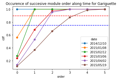
For Gariguette varieties
[13]:
Gariguette_frequency = occurence_module_order_along_time(data= Gariguette_extraction_at_module_scale,frequency_type= "cdf")
Gariguette_frequency
[13]:
| date | 2014/12/10 | 2015/01/08 | 2015/02/12 | 2015/03/06 | 2015/04/02 | 2015/05/19 |
|---|---|---|---|---|---|---|
| order | ||||||
| 0 | 1.0 | 0.5625 | 0.272727 | 0.236842 | 0.136364 | 0.113924 |
| 1 | 1.0 | 1.0000 | 1.000000 | 0.684211 | 0.530303 | 0.367089 |
| 2 | 1.0 | 1.0000 | 1.000000 | 0.973684 | 0.954545 | 0.658228 |
| 3 | 1.0 | 1.0000 | 1.000000 | 1.000000 | 1.000000 | 0.873418 |
| 4 | 1.0 | 1.0000 | 1.000000 | 1.000000 | 1.000000 | 0.987342 |
| 5 | 1.0 | 1.0000 | 1.000000 | 1.000000 | 1.000000 | 1.000000 |
[14]:
Gariguette_frequency.plot.line(marker = "o")
plt.axhline(y = 0.9, color = "r",linestyle="--") # threshold at 0.9 quartile,
plt.axhline(y = 0.75, color = "b",linestyle="--") # threshold at 0.75 quartile
plt.title("Occurence of succesive module order along time for Gariguette")
plt.ylabel("cdf")
[14]:
Text(0, 0.5, 'cdf')
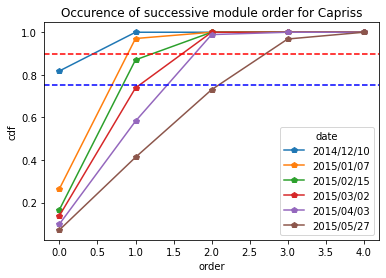
For Capriss varieties
[15]:
Capriss_frequency = occurence_module_order_along_time(data= Capriss_extraction_at_module_scale,frequency_type= "cdf")
Capriss_frequency
[15]:
| date | 2014/12/10 | 2015/01/07 | 2015/02/15 | 2015/03/02 | 2015/04/03 | 2015/05/27 |
|---|---|---|---|---|---|---|
| order | ||||||
| 0 | 0.818182 | 0.264706 | 0.166667 | 0.138462 | 0.098901 | 0.071429 |
| 1 | 1.000000 | 0.970588 | 0.870370 | 0.738462 | 0.582418 | 0.412698 |
| 2 | 1.000000 | 1.000000 | 1.000000 | 1.000000 | 0.989011 | 0.730159 |
| 3 | 1.000000 | 1.000000 | 1.000000 | 1.000000 | 1.000000 | 0.968254 |
| 4 | 1.000000 | 1.000000 | 1.000000 | 1.000000 | 1.000000 | 1.000000 |
[16]:
Capriss_frequency.plot.line(marker = "p")
plt.axhline(y = 0.9, color = "r",linestyle="--") # threshold at 0.9 quartile,
plt.axhline(y = 0.75, color = "b",linestyle="--") # threshold at 0.75 quartile
plt.title("Occurence of successive module order for Capriss")
plt.ylabel("cdf")
[16]:
Text(0, 0.5, 'cdf')
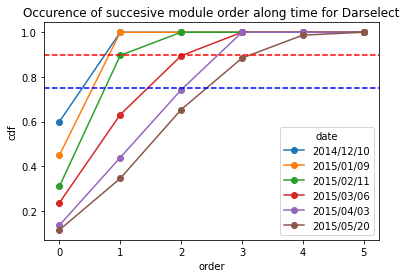
** For Darselect variety**
[17]:
Darselect_frequency = occurence_module_order_along_time(data= Darselect_extraction_at_module_scale,frequency_type= "cdf")
Darselect_frequency
[17]:
| date | 2014/12/10 | 2015/01/09 | 2015/02/11 | 2015/03/06 | 2015/04/03 | 2015/05/20 |
|---|---|---|---|---|---|---|
| order | ||||||
| 0 | 0.6 | 0.45 | 0.310345 | 0.236842 | 0.136364 | 0.115385 |
| 1 | 1.0 | 1.00 | 0.896552 | 0.631579 | 0.439394 | 0.346154 |
| 2 | 1.0 | 1.00 | 1.000000 | 0.894737 | 0.742424 | 0.653846 |
| 3 | 1.0 | 1.00 | 1.000000 | 1.000000 | 1.000000 | 0.884615 |
| 4 | 1.0 | 1.00 | 1.000000 | 1.000000 | 1.000000 | 0.987179 |
| 5 | 1.0 | 1.00 | 1.000000 | 1.000000 | 1.000000 | 1.000000 |
[18]:
Darselect_frequency.plot.line(marker = "o")
plt.axhline(y = 0.9, color = "r",linestyle="--") # threshold at 0.9 quartile,
plt.axhline(y = 0.75, color = "b",linestyle="--") # threshold at 0.75 quartile
plt.title("Occurence of succesive module order along time for Darselect")
plt.ylabel("cdf")
[18]:
Text(0, 0.5, 'cdf')
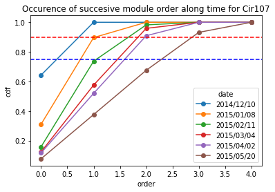
** For Cir107 Variety**
[19]:
Cir107_frequency = occurence_module_order_along_time(data= Cir107_extraction_at_module_scale,frequency_type= "cdf")
Cir107_frequency
[19]:
| date | 2014/12/10 | 2015/01/08 | 2015/02/11 | 2015/03/04 | 2015/04/02 | 2015/05/20 |
|---|---|---|---|---|---|---|
| order | ||||||
| 0 | 0.642857 | 0.310345 | 0.157895 | 0.123288 | 0.116883 | 0.076923 |
| 1 | 1.000000 | 0.896552 | 0.736842 | 0.575342 | 0.519481 | 0.376068 |
| 2 | 1.000000 | 1.000000 | 0.982456 | 0.958904 | 0.909091 | 0.675214 |
| 3 | 1.000000 | 1.000000 | 1.000000 | 1.000000 | 1.000000 | 0.931624 |
| 4 | 1.000000 | 1.000000 | 1.000000 | 1.000000 | 1.000000 | 1.000000 |
[20]:
Cir107_frequency.plot.line(marker = "o")
plt.axhline(y = 0.9, color = "r",linestyle="--") # threshold at 0.9 quartile,
plt.axhline(y = 0.75, color = "b",linestyle="--") # threshold at 0.75 quartile
plt.title("Occurence of succesive module order along time for Cir107")
plt.ylabel("cdf")
[20]:
Text(0, 0.5, 'cdf')
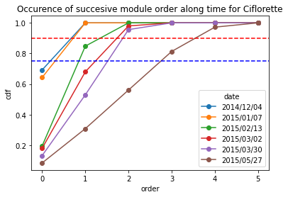
**For Ciflorette variety **
[21]:
Ciflorette_frequency = occurence_module_order_along_time(data= Ciflorette_extraction_at_module_scale,frequency_type= "cdf")
Ciflorette_frequency
[21]:
| date | 2014/12/04 | 2015/01/07 | 2015/02/13 | 2015/03/02 | 2015/03/30 | 2015/05/27 |
|---|---|---|---|---|---|---|
| order | ||||||
| 0 | 0.692308 | 0.642857 | 0.195652 | 0.18 | 0.132353 | 0.084112 |
| 1 | 1.000000 | 1.000000 | 0.847826 | 0.68 | 0.529412 | 0.308411 |
| 2 | 1.000000 | 1.000000 | 1.000000 | 0.98 | 0.955882 | 0.560748 |
| 3 | 1.000000 | 1.000000 | 1.000000 | 1.00 | 1.000000 | 0.813084 |
| 4 | 1.000000 | 1.000000 | 1.000000 | 1.00 | 1.000000 | 0.971963 |
| 5 | 1.000000 | 1.000000 | 1.000000 | 1.00 | 1.000000 | 1.000000 |
[22]:
Ciflorette_frequency.plot.line(marker = "o")
plt.axhline(y = 0.9, color = "r",linestyle="--") # threshold at 0.9 quartile,
plt.axhline(y = 0.75, color = "b",linestyle="--") # threshold at 0.75 quartile
plt.title("Occurence of succesive module order along time for Ciflorette")
plt.ylabel("cdf")
[22]:
Text(0, 0.5, 'cdf')
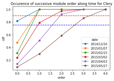
For Clery variety
[23]:
Clery_frequency = occurence_module_order_along_time(data= Clery_extraction_at_module_scale,frequency_type= "cdf")
Clery_frequency
[23]:
| date | 2014/12/10 | 2015/01/07 | 2015/02/15 | 2015/03/02 | 2015/04/03 | 2015/05/27 |
|---|---|---|---|---|---|---|
| order | ||||||
| 0 | 0.818182 | 0.473684 | 0.310345 | 0.236842 | 0.138462 | 0.089109 |
| 1 | 1.000000 | 1.000000 | 1.000000 | 0.789474 | 0.507692 | 0.297030 |
| 2 | 1.000000 | 1.000000 | 1.000000 | 0.973684 | 0.923077 | 0.584158 |
| 3 | 1.000000 | 1.000000 | 1.000000 | 1.000000 | 1.000000 | 0.861386 |
| 4 | 1.000000 | 1.000000 | 1.000000 | 1.000000 | 1.000000 | 1.000000 |
[24]:
Clery_frequency.plot.line(marker = "o")
plt.axhline(y = 0.9, color = "r",linestyle="--") # threshold at 0.9 quartile,
plt.axhline(y = 0.75, color = "b",linestyle="--") # threshold at 0.75 quartile
plt.title("Occurence of succesive module order along time for Clery")
plt.ylabel("cdf")
[24]:
Text(0, 0.5, 'cdf')
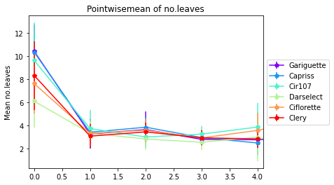
3.4.2. Pointwise mean no. Leaves, Flowers, Stolon by module order
The first step is calcul mean and standard deviation for each variable by genotype and order
[25]:
Mean= All_varieties_extraction_at_module_scale.groupby(["Genotype", "order"]).mean()
sd= All_varieties_extraction_at_module_scale.groupby(["Genotype", "order"]).std()
3.4.2.1. Pointwise mean no. leaves by module order and génotype
[26]:
pointwisemean_plot(data_mean=Mean,
                   data_sd=sd,
                   varieties=["Gariguette","Capriss","Cir107","Darselect","Ciflorette", "Clery"],
                   variable='nb_total_leaves',
                   title= "Pointwisemean of no.leaves",
                   ylab="Mean no.leaves",
                   expand= 0.1)
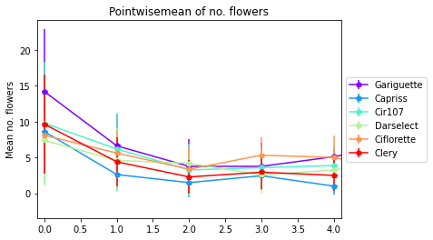
3.4.2.2. Pointwise mean of no. total flowers by genotype and orders
[27]:
pointwisemean_plot(data_mean=Mean,
                   data_sd=sd,
                   varieties=["Gariguette","Capriss","Cir107","Darselect","Ciflorette", "Clery"],
                   variable='nb_total_flowers',
                   title= "Pointwisemean of no. flowers",
                   ylab="Mean no. flowers",
                   expand= 0.1)
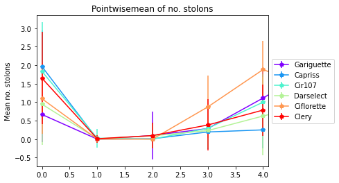
3.4.3. Number of stolons by module orders
[28]:
pointwisemean_plot(data_mean=Mean,
                   data_sd=sd,
                   varieties=["Gariguette","Capriss","Cir107","Darselect","Ciflorette", "Clery"],
                   variable='nb_stolons',
                   title= "Pointwisemean of no. stolons",
                   ylab="Mean no. stolons", expand=0.1)
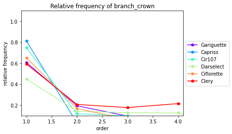
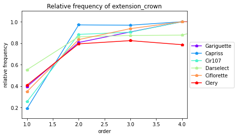
3.4.4. Type of Crowns (Extension crown vs Branch crowns)
[29]:
crowntype_distribution(data= All_varieties_extraction_at_module_scale, varieties=["Gariguette","Capriss","Cir107","Darselect","Ciflorette","Clery"],crown_type="branch_crown",expand=0.1)
<matplotlib.colors.LinearSegmentedColormap object at 0x7f5a5d00b550>
[29]:
| Main | extension_crown | branch_crown | ||
|---|---|---|---|---|
| Genotype | order | |||
| Capriss | 1 | 0.0 | 0.189474 | 0.810526 |
| Capriss | 2 | 0.0 | 0.970588 | 0.029412 |
| Capriss | 3 | 0.0 | 0.967742 | 0.032258 |
| Capriss | 4 | 0.0 | 1.000000 | 0.000000 |
| Ciflorette | 1 | 0.0 | 0.347826 | 0.652174 |
| Ciflorette | 2 | 0.0 | 0.833333 | 0.166667 |
| Ciflorette | 3 | 0.0 | 0.935484 | 0.064516 |
| Ciflorette | 4 | 0.0 | 1.000000 | 0.000000 |
| Ciflorette | 5 | 0.0 | 1.000000 | 0.000000 |
| Cir107 | 1 | 0.0 | 0.253247 | 0.746753 |
| Cir107 | 2 | 0.0 | 0.881818 | 0.118182 |
| Cir107 | 3 | 0.0 | 0.902439 | 0.097561 |
| Cir107 | 4 | 0.0 | 1.000000 | 0.000000 |
| Clery | 1 | 0.0 | 0.408163 | 0.591837 |
| Clery | 2 | 0.0 | 0.793651 | 0.206349 |
| Clery | 3 | 0.0 | 0.823529 | 0.176471 |
| Clery | 4 | 0.0 | 0.785714 | 0.214286 |
| Darselect | 1 | 0.0 | 0.551724 | 0.448276 |
| Darselect | 2 | 0.0 | 0.859649 | 0.140351 |
| Darselect | 3 | 0.0 | 0.871795 | 0.128205 |
| Darselect | 4 | 0.0 | 0.875000 | 0.125000 |
| Darselect | 5 | 0.0 | 1.000000 | 0.000000 |
| Gariguette | 1 | 0.0 | 0.393617 | 0.606383 |
| Gariguette | 2 | 0.0 | 0.806452 | 0.193548 |
| Gariguette | 3 | 0.0 | 0.904762 | 0.095238 |
| Gariguette | 4 | 0.0 | 1.000000 | 0.000000 |
| Gariguette | 5 | 0.0 | 1.000000 | 0.000000 |
[30]:
crowntype_distribution(data= All_varieties_extraction_at_module_scale, varieties=["Gariguette","Capriss","Cir107","Darselect","Ciflorette","Clery"],crown_type="extension_crown",expand=0.1,plot=True)
<matplotlib.colors.LinearSegmentedColormap object at 0x7f5a5cfbe130>
[30]:
| Main | extension_crown | branch_crown | ||
|---|---|---|---|---|
| Genotype | order | |||
| Capriss | 1 | 0.0 | 0.189474 | 0.810526 |
| Capriss | 2 | 0.0 | 0.970588 | 0.029412 |
| Capriss | 3 | 0.0 | 0.967742 | 0.032258 |
| Capriss | 4 | 0.0 | 1.000000 | 0.000000 |
| Ciflorette | 1 | 0.0 | 0.347826 | 0.652174 |
| Ciflorette | 2 | 0.0 | 0.833333 | 0.166667 |
| Ciflorette | 3 | 0.0 | 0.935484 | 0.064516 |
| Ciflorette | 4 | 0.0 | 1.000000 | 0.000000 |
| Ciflorette | 5 | 0.0 | 1.000000 | 0.000000 |
| Cir107 | 1 | 0.0 | 0.253247 | 0.746753 |
| Cir107 | 2 | 0.0 | 0.881818 | 0.118182 |
| Cir107 | 3 | 0.0 | 0.902439 | 0.097561 |
| Cir107 | 4 | 0.0 | 1.000000 | 0.000000 |
| Clery | 1 | 0.0 | 0.408163 | 0.591837 |
| Clery | 2 | 0.0 | 0.793651 | 0.206349 |
| Clery | 3 | 0.0 | 0.823529 | 0.176471 |
| Clery | 4 | 0.0 | 0.785714 | 0.214286 |
| Darselect | 1 | 0.0 | 0.551724 | 0.448276 |
| Darselect | 2 | 0.0 | 0.859649 | 0.140351 |
| Darselect | 3 | 0.0 | 0.871795 | 0.128205 |
| Darselect | 4 | 0.0 | 0.875000 | 0.125000 |
| Darselect | 5 | 0.0 | 1.000000 | 0.000000 |
| Gariguette | 1 | 0.0 | 0.393617 | 0.606383 |
| Gariguette | 2 | 0.0 | 0.806452 | 0.193548 |
| Gariguette | 3 | 0.0 | 0.904762 | 0.095238 |
| Gariguette | 4 | 0.0 | 1.000000 | 0.000000 |
| Gariguette | 5 | 0.0 | 1.000000 | 0.000000 |
3.4.5. Distribution of complete vs complete module as function of module order
3.4.6. As fonction of module orders
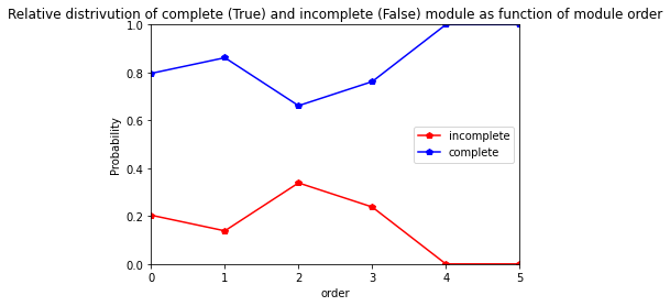
** For Gariguette variety**
[31]:
res=pd.crosstab(index= Gariguette_extraction_at_module_scale["order"], columns= Gariguette_extraction_at_module_scale["complete_module"],normalize="index")
res.columns = ["incomplete","complete"]
res
[31]:
| incomplete | complete | |
|---|---|---|
| order | ||
| 0 | 0.203704 | 0.796296 |
| 1 | 0.138298 | 0.861702 |
| 2 | 0.338710 | 0.661290 |
| 3 | 0.238095 | 0.761905 |
| 4 | 0.000000 | 1.000000 |
| 5 | 0.000000 | 1.000000 |
[32]:
res.plot.line(marker="p", color=["red","blue"])
plt.axis([0,5,0,1])
plt.ylabel("Probability")
plt.title("Relative distrivution of complete (True) and incomplete (False) module as function of module order")
[32]:
Text(0.5, 1.0, 'Relative distrivution of complete (True) and incomplete (False) module as function of module order')
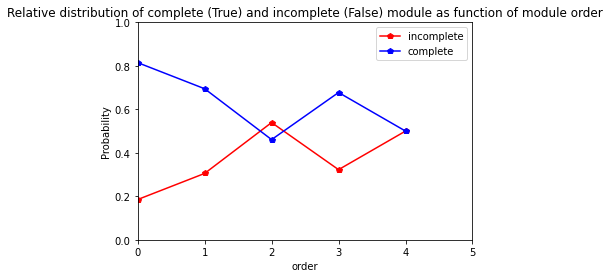
For Capriss variety
[33]:
res=pd.crosstab(index= Capriss_extraction_at_module_scale["order"], columns= Capriss_extraction_at_module_scale["complete_module"],normalize="index")
res.columns = ["incomplete","complete"]
res
[33]:
| incomplete | complete | |
|---|---|---|
| order | ||
| 0 | 0.185185 | 0.814815 |
| 1 | 0.305263 | 0.694737 |
| 2 | 0.539216 | 0.460784 |
| 3 | 0.322581 | 0.677419 |
| 4 | 0.500000 | 0.500000 |
[34]:
res.plot.line(marker="p",color= ["red", "blue"])
plt.axis([0,5,0,1])
plt.ylabel("Probability")
plt.title("Relative distribution of complete (True) and incomplete (False) module as function of module order")
[34]:
Text(0.5, 1.0, 'Relative distribution of complete (True) and incomplete (False) module as function of module order')
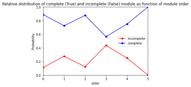
For Darselect variety
[35]:
res=pd.crosstab(index= Darselect_extraction_at_module_scale["order"], columns= Darselect_extraction_at_module_scale["complete_module"],normalize="index")
res.columns = ["incomplete","complete"]
res
[35]:
| incomplete | complete | |
|---|---|---|
| order | ||
| 0 | 0.111111 | 0.888889 |
| 1 | 0.275862 | 0.724138 |
| 2 | 0.122807 | 0.877193 |
| 3 | 0.435897 | 0.564103 |
| 4 | 0.250000 | 0.750000 |
| 5 | 0.000000 | 1.000000 |
[36]:
res.plot.line(marker="p",color= ["red", "blue"])
plt.axis([0,5,0,1])
plt.ylabel("Probability")
plt.title("Relative distribution of complete (True) and incomplete (False) module as function of module order")
[36]:
Text(0.5, 1.0, 'Relative distribution of complete (True) and incomplete (False) module as function of module order')
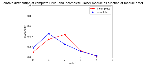
For Cir107 variety
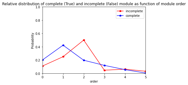
[37]:
res=pd.crosstab(index=Cir107_extraction_at_module_scale["order"], columns= Cir107_extraction_at_module_scale["complete_module"],normalize="columns")
res.columns = ["incomplete","complete"]
res
[37]:
| incomplete | complete | |
|---|---|---|
| order | ||
| 0 | 0.088235 | 0.169811 |
| 1 | 0.343137 | 0.449057 |
| 2 | 0.431373 | 0.249057 |
| 3 | 0.117647 | 0.109434 |
| 4 | 0.019608 | 0.022642 |
[38]:
res.plot.line(marker="p",color= ["red", "blue"])
plt.axis([0,5,0,1])
plt.ylabel("Probability")
plt.title("Relative distribution of complete (True) and incomplete (False) module as function of module order")
[38]:
Text(0.5, 1.0, 'Relative distribution of complete (True) and incomplete (False) module as function of module order')
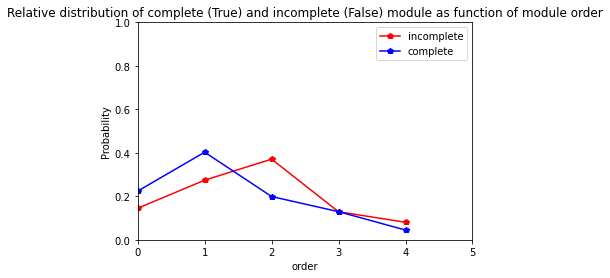
For Ciflorette variety
[39]:
res=pd.crosstab(index=Ciflorette_extraction_at_module_scale["order"], columns= Ciflorette_extraction_at_module_scale["complete_module"],normalize="columns")
res.columns = ["incomplete","complete"]
res
[39]:
| incomplete | complete | |
|---|---|---|
| order | ||
| 0 | 0.109375 | 0.200855 |
| 1 | 0.250000 | 0.423077 |
| 2 | 0.500000 | 0.196581 |
| 3 | 0.046875 | 0.119658 |
| 4 | 0.062500 | 0.055556 |
| 5 | 0.031250 | 0.004274 |
[40]:
res.plot.line(marker="p",color= ["red", "blue"])
plt.axis([0,5,0,1])
plt.ylabel("Probability")
plt.title("Relative distribution of complete (True) and incomplete (False) module as function of module order")
[40]:
Text(0.5, 1.0, 'Relative distribution of complete (True) and incomplete (False) module as function of module order')
For Clery variety
[41]:
res=pd.crosstab(index=Clery_extraction_at_module_scale["order"], columns= Clery_extraction_at_module_scale["complete_module"],normalize="columns")
res.columns = ["incomplete","complete"]
res
[41]:
| incomplete | complete | |
|---|---|---|
| order | ||
| 0 | 0.145161 | 0.223881 |
| 1 | 0.274194 | 0.402985 |
| 2 | 0.370968 | 0.199005 |
| 3 | 0.129032 | 0.129353 |
| 4 | 0.080645 | 0.044776 |
[42]:
res.plot.line(marker="p",color= ["red", "blue"])
plt.axis([0,5,0,1])
plt.ylabel("Probability")
plt.title("Relative distribution of complete (True) and incomplete (False) module as function of module order")
[42]:
Text(0.5, 1.0, 'Relative distribution of complete (True) and incomplete (False) module as function of module order')
3.4.7. As fonction of date
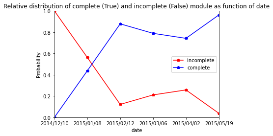
** Gariguette**
[43]:
res=pd.crosstab(index=Gariguette_extraction_at_module_scale["date"], columns= Gariguette_extraction_at_module_scale["complete_module"],normalize="index")
res.columns = ["incomplete","complete"]
res
[43]:
| incomplete | complete | |
|---|---|---|
| date | ||
| 2014/12/10 | 1.000000 | 0.000000 |
| 2015/01/08 | 0.562500 | 0.437500 |
| 2015/02/12 | 0.121212 | 0.878788 |
| 2015/03/06 | 0.210526 | 0.789474 |
| 2015/04/02 | 0.257576 | 0.742424 |
| 2015/05/19 | 0.037975 | 0.962025 |
[44]:
res.plot.line(marker="p",color= ["red", "blue"])
plt.axis([0,5,0,1])
plt.ylabel("Probability")
plt.title("Relative distribution of complete (True) and incomplete (False) module as function of date")
[44]:
Text(0.5, 1.0, 'Relative distribution of complete (True) and incomplete (False) module as function of date')
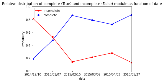
Capriss
[45]:
res=pd.crosstab(index=Capriss_extraction_at_module_scale["date"], columns= Capriss_extraction_at_module_scale["complete_module"],normalize="index")
res.columns = ["incomplete","complete"]
res
[45]:
| incomplete | complete | |
|---|---|---|
| date | ||
| 2014/12/10 | 1.000000 | 0.000000 |
| 2015/01/07 | 0.735294 | 0.264706 |
| 2015/02/15 | 0.388889 | 0.611111 |
| 2015/03/02 | 0.476923 | 0.523077 |
| 2015/04/03 | 0.362637 | 0.637363 |
| 2015/05/27 | 0.111111 | 0.888889 |
[46]:
res.plot.line(marker="p",color= ["red", "blue"])
plt.axis([0,5,0,1])
plt.ylabel("Probability")
plt.title("Relative distribution of complete (True) and incomplete (False) module as function of date")
[46]:
Text(0.5, 1.0, 'Relative distribution of complete (True) and incomplete (False) module as function of date')
Darselect
[47]:
res=pd.crosstab(index=Capriss_extraction_at_module_scale["date"], columns= Capriss_extraction_at_module_scale["complete_module"],normalize="index")
res.columns = ["incomplete","complete"]
res
[47]:
| incomplete | complete | |
|---|---|---|
| date | ||
| 2014/12/10 | 1.000000 | 0.000000 |
| 2015/01/07 | 0.735294 | 0.264706 |
| 2015/02/15 | 0.388889 | 0.611111 |
| 2015/03/02 | 0.476923 | 0.523077 |
| 2015/04/03 | 0.362637 | 0.637363 |
| 2015/05/27 | 0.111111 | 0.888889 |
[48]:
res.plot.line(marker="p",color= ["red", "blue"])
plt.axis([0,5,0,1])
plt.ylabel("Probability")
plt.title("Relative distribution of complete (True) and incomplete (False) module as function of date")
[48]:
Text(0.5, 1.0, 'Relative distribution of complete (True) and incomplete (False) module as function of date')

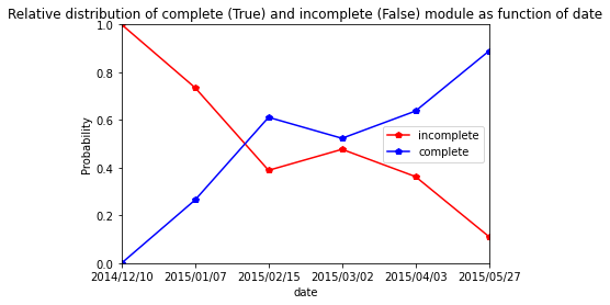
Cir107
[49]:
res=pd.crosstab(index=Cir107_extraction_at_module_scale["date"], columns= Cir107_extraction_at_module_scale["complete_module"],normalize="index")
res.columns = ["incomplete","complete"]
res
[49]:
| incomplete | complete | |
|---|---|---|
| date | ||
| 2014/12/10 | 0.928571 | 0.071429 |
| 2015/01/08 | 0.482759 | 0.517241 |
| 2015/02/11 | 0.263158 | 0.736842 |
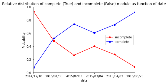
| 2015/03/04 | 0.397260 | 0.602740 |
| 2015/04/02 | 0.272727 | 0.727273 |
| 2015/05/20 | 0.085470 | 0.914530 |
[50]:
res.plot.line(marker="p",color= ["red", "blue"])
plt.axis([0,5,0,1])
plt.ylabel("Probability")
plt.title("Relative distribution of complete (True) and incomplete (False) module as function of date")
[50]:
Text(0.5, 1.0, 'Relative distribution of complete (True) and incomplete (False) module as function of date')
Ciflorette
[51]:
res=pd.crosstab(index=Ciflorette_extraction_at_module_scale["date"], columns= Ciflorette_extraction_at_module_scale["complete_module"],normalize="index")
res.columns = ["incomplete","complete"]
res
[51]:
| incomplete | complete | |
|---|---|---|
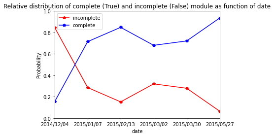
| date | ||
| 2014/12/04 | 0.846154 | 0.153846 |
| 2015/01/07 | 0.285714 | 0.714286 |
| 2015/02/13 | 0.152174 | 0.847826 |
| 2015/03/02 | 0.320000 | 0.680000 |
| 2015/03/30 | 0.279412 | 0.720588 |
| 2015/05/27 | 0.065421 | 0.934579 |
[52]:
res.plot.line(marker="p",color= ["red", "blue"])
plt.axis([0,5,0,1])
plt.ylabel("Probability")
plt.title("Relative distribution of complete (True) and incomplete (False) module as function of date")
[52]:
Text(0.5, 1.0, 'Relative distribution of complete (True) and incomplete (False) module as function of date')
Clery
[53]:
res=pd.crosstab(index=Clery_extraction_at_module_scale["date"], columns= Clery_extraction_at_module_scale["complete_module"],normalize="index")
res.columns = ["incomplete","complete"]
res
[53]:
| incomplete | complete | |
|---|---|---|
| date | ||
| 2014/12/10 | 0.818182 | 0.181818 |
| 2015/01/07 | 0.526316 | 0.473684 |
| 2015/02/15 | 0.137931 | 0.862069 |
| 2015/03/02 | 0.210526 | 0.789474 |
| 2015/04/03 | 0.276923 | 0.723077 |
| 2015/05/27 | 0.128713 | 0.871287 |
[54]:
res.plot.line(marker="p",color= ["red", "blue"])
plt.axis([0,5,0,1])
plt.ylabel("Probability")
plt.title("Relative distribution of complete (True) and incomplete (False) module as function of date")
[54]:
Text(0.5, 1.0, 'Relative distribution of complete (True) and incomplete (False) module as function of date')